Brief Matrix Algebra Review

Matrix algebra is a form of mathematics that allows compact notation for, and mathematical
manipulation of, high-dimensional expressions and equations. For the purposes of this
class, only a relatively simple exposition is required, in order to understand the notation for
multivariate equations and calculations.

1 Matrix Notation

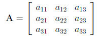
The basic unit in matrix algebra is a matrix, generally expressed as:
(1)
Here, the matrix A is denoted as a matrix by the boldfaced type. Matrices are also
often denoted using bold-faced type. Matrices can be of any dimension; in this example,
the matrix is a '3-by-3'or '3 × 3'matrix. The number of rows is listed first; the number of
columns is listed second. The subscripts of the matrix elements (a's) clarify this: the 3rd
item in the second row is element a₂₃. A matrix with only one element (i.e., 1 × 1 dimension)
is called a scalar. A matrix with only a single column is called a column vector; a matrix
with only a single row is called a row vector. The term 'vector' also has meaning in analytic
geometry, referring to a line segment that originates at the origin (0, 0, . . . 0) and terminates
at the coordinates listed in the k dimensions. For example, you are already familiar with the
Cartesian coordinate (4, 5), which is located 4 units from 0 in the x dimension and 5 units
from 0 in the y dimension. The vector [4, 5], then, is the line segment formed by taking a
straight line from (0, 0) to (4, 5).

2 Matrix Operations

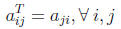
The first important operation that can be performed on a matrix (or vector) is the transpose
function, denoted as: A' or A^T. The transpose function reverses the rows and columns of a
matrix so that:
(2)

This equation says that the i, j−th element of the transposed matrix is the j, i−th element
of the original element for all i = 1 . . . I and j = 1 . . . J elements. The dimensionality of a
transposed matrix, therefore, is the opposite of the original matrix. For example, if matrix
B is 3 × 2, then matrix B^T will be of dimension 2 × 3.

With this basic function developed, we can now discuss other matrix functions, including
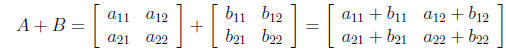
matrix addition, subtraction, and multiplication (including division). Matrix addition and
subtraction are simple. Provided two matrices have the same dimensionality, the addition
or subtraction of two matrices proceeds by simply adding and subtracting corresponding
elements in the two matrices:
(3)

The commutative property of addition and subtraction that holds in scalar algebra also
holds in matrix algebra: the order of addition or subtraction of matrices makes no difference
to the outcome, so that A + B + C = C + B + A.

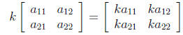
Matrix multiplication is slightly more difficult than addition and subtraction, unless one
is multiplying a matrix by a scalar. In that case, the scalar is distributed to each element in
the matrix, and multiplication is carried out element by element:
(4)

In the event two matrices are being multiplied, before multiplying, one must make sure
the matrices 'conform' for multiplication. This means that the number of columns in the
first matrix must equal the number of rows in the second matrix. For example, one can not
post-multiply a 2 × 3 matrix A by another 2 × 3 matrix B , because the number of columns
in A is 3, while the number of rows in B is 2. One could however multiply A by a 3 × 2
matrix C. The matrix that results from multiplying A and C would have dimension 2 × 2
(same number of rows as the first matrix; same number of columns as the second matrix).
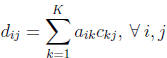
The general rule for matrix multiplication is as follows: if one is multiplying A × C = D,
then:
(5)

This says that the ij −th element of matrix D is equal to the sum of the multiple of the
elements in row i of A and the column j of C . Matrix multiplication is thus a fairly tedious
process. As an example, assume A is 2 ×3 and C is 3 ×2, with the following elements:
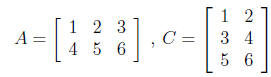(6)

Then, element d11 = (1 × 1) + (2 × 3) + (3 × 5) = 22, and the entire D matrix is (solve
this yourself):
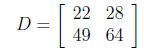(7)
Notice that D is 2 × 2.

Unlike matrix addition and subtraction, in which order of the matrices is irrelevant, order
matters for multiplication. Obviously, given the conformability requirement, reversing the
order of matrices may make multiplication impossible (e.g., while a 3 × 2 matrix can be
post-multiplied by a 2 × 4 matrix, the 2 × 4 matrix can NOT be post-multiplied by the 3 × 2
matrix). However, even if matrices are conformable for multiplication after reversing their
order, the resulting matrices will not generally be identical. For example, a 1 × k row vector
multiplied by a k × 1 column vector will yield a scalar (1?), but if we reverse the order of
multiplication, we will obtain a k × k matrix.

Some additional functions that apply to matrices and are commonly seen include the
trace operator (the trace of A is denoted TrA), the determinant, and the inverse. The trace
of a matrix is simply the sum of the diagonal elements of the matrix. The determinant is
more difficult. Technically, the determinant is the sum of the signed multiples of all the
permutations of a matrix, where 'permutations' refer to the unique combinations of a single
element from each row and column, for all rows and columns. If d denotes the dimensionality
of a matrix, then there are d! permutations for the matrix. For instance, in a 3 × 3 matrix,
there are a total of 6 permutations (3! = 3 × 2 ×1 = 6): (a₁₁, a₂₂, a₃₃), (a₁₂, a₂₃, a₃₁), (a₁₃,
a₂₁, a₃₂), (a₁₃, a₂₂, a₃₁), (a₁₁, a₂₃, a₃₂), (a₁₂, a₂₁, a₃₃). Notice how for each combination, there
is one element from each row and column. The signing of each permutation is determined
by the column position of each element in all the pairs that can be constructed using the
elements of the permutation, and the subscript of element at each position in each pair.
For example, the permutation (a₁₁, a₂₂, a₃₃) has elements from columns 1,2, and 3. The
possible ordered (i, j) pairs that can come from this permutation include (1, 2), (1, 3), and
(2, 3) (based on the column position). If there are an even number of (i, j) pairs in which
i > j, then the permutation is considered even and takes a positive sign; otherwise, the
permutation is considered odd and takes a negative sign. In this example, there are 0 pairs
in which i > j, so the permutation is even (0 is even). However, in the permutation (a₁₃,
a₂₂, a₃₁), the pairs are (3, 2), (3, 1), and (2, 1). In this set, all three pairs are such that i > j,
hence this permutation is odd and takes a negative sign. The determinant is denoted using
absolute value bars on either side of the matrix name: for instance, the determinant of A is
denoted as |A|.

For 2 × 2 and 3 × 3 matrices, determinants can be calculated fairly easily; however, for
larger matrices, the number of permutations becomes large rapidly. Fortunately, several
rules simplify the process. First, if any row or column in a matrix is a vector of 0, then the
determinant is 0. In that case, the matrix is said not to be 'of full rank'. Second, the same
is true if any two rows or columns is identical. Third, for a diagonal matrix (i.e., there are
0s everywhere but the main diagonal-the 11, 22, 33,... positions), the determinant is only
the multiple of the diagonal elements. There are additional rules, but they are not necessary
for this brief introduction. We will note that the determinant is essentially a measure of the
area/volume/hypervolume bounded by the vectors of the matrix. This helps, we think, to
clarify why matrices with 0 vectors in them have determinant 0: just as in two dimensions
a line has no area, when we have a 0 vector in a matrix, the dimensionality of the figure
bounded by the matrix is reduced by a dimension (because one vector doesn't pass the
origin), and hence the hypervolume is necessarily 0.

Finally, a very important function for matrix algebra is the inverse function. The inverse
function allows the matrix equivalent of division. In a sense, just as 5 times its inverse
1/5 = 1, a matrix A times its inverse-denoted A^-1-equals I, where I is the 'identity matrix'. A
n identity matrix is a diagonal matrix with ones along the diagonal. It is the matrix
equivalent of unity (1). Some simple algebraic rules follow from the discussion of inverses
and the identity matrix:
AA^-1 = A^-1A = I  (8)

Furthermore,
AI = IA = A  (9)

Given the commutability implicit in the above rules, it stands that inverses only exist
for square matrices, and that all identity matrices are square matrices. For that matter, the
determinant function can only apply to square matrices also.

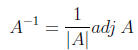
Computing the inverse of matrices is a difficult task, and there are several methods by
which to derive them. Probably the simplest method to compute an inverse is to use the
following formula:
(10)

The only new element in this formula is the adj A , which means 'adjoint of A .' The
adjoint of a matrix is the transpose of its matrix of cofactors, where a cofactor is the signed
determinant of the 'minor' of an element of a matrix. The minor of element i, j can be found
by deleting the ith row and jth column of the matrix. For example, the minor of element
a₁₁ of the matrix A above is:
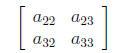(11)

Taking its determinant leaves one with a scalar that is then signed (by multiplying by
−1^i+j). In this case, we obtain (−1)²(a₂₂a₃₃ −a₂₃a₃₂) as the cofactor for element a₁₁. If one
replaces every element in matrix A with its signed cofactor, then transposes the result, one
will obtain the adjoint of A . Multiplying this by 1/|A| (a scalar) will yield the inverse of A .
There are a number of important properties of cofactors that enable more rapid computation
of determinants, but discussing these is beyond the scope of this simple introduction.

Fortunately, computer packages tend to have determinant and inversion routines built
into them, and there are plenty of inversion algorithms available if you are designing your
own software, so that we generally need not worry. It is worth mentioning that if a matrix
has a 0 determinant, it does not have an inverse. There are many additional matrix algebra
rules and tricks that one may need to know; however, they are also beyond the scope of this
introduction.

3 The OLS Regression Solution in Matrix Form

We close this section by demonstrating the utility of matrix algebra in a statistical problem:
the OLS regression solution.

When dealing with the OLS regression problem, we can think of the entire data set in
matrix terms:

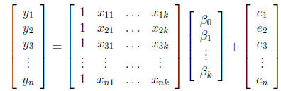(12)
In this problem, there are n individuals in the dataset measured on one dependent (outcome)
variable y, with k regressor (predictor) variables x, and hence k coefficients to be
estimated. The column of ones represents the intercept. If one performs the matrix algebra
(multiplication) for the first observation, y₁, one can see that:
(13)

which is exactly as it should be: the dependent variable for observation 1 is a linear
combination of the individual's values on the regressors weighted by the regression coefficients,
plus an individual-specific error term. This equation can be written more succinctly
by simply writing:
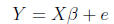(14)

How can we solve for ? Just as in scalar algebra, we need to isolate . Unlike scalar
algebra, however, we can't simply subtract the error term from both sides and divide by X,
because a) there is no matrix division, really, and b) multiplication must conform. So, we
first multiply both sides by
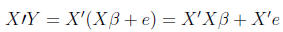(15)

We multiply by the transpose of X here, because X^-1Y would not conform for multiplication.
One of the assumptions of OLS regression says that X and e are uncorrelated, hence
Thus, we are left with:
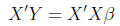(16)

From here, we need to eliminate from the right side of the equation. We can do
this if we take the inverse of and multiply both sides of the equation by it:
(17)

This follows, because A^-1A = I and IA = A. Thus, the OLS solution for is
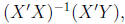which should look familiar.